8. Stationarity and Ergodicity
In addition to what’s in Anaconda, this lecture will need the following libraries:
!pip install quantecon
Requirement already satisfied: quantecon in /usr/share/miniconda3/envs/quantecon/lib/python3.8/site-packages (0.5.2)
Requirement already satisfied: requests in /usr/share/miniconda3/envs/quantecon/lib/python3.8/site-packages (from quantecon) (2.26.0)
Requirement already satisfied: scipy>=1.0.0 in /usr/share/miniconda3/envs/quantecon/lib/python3.8/site-packages (from quantecon) (1.7.1)
Requirement already satisfied: numpy in /usr/share/miniconda3/envs/quantecon/lib/python3.8/site-packages (from quantecon) (1.20.3)
Requirement already satisfied: sympy in /usr/share/miniconda3/envs/quantecon/lib/python3.8/site-packages (from quantecon) (1.9)
Requirement already satisfied: numba>=0.38 in /usr/share/miniconda3/envs/quantecon/lib/python3.8/site-packages (from quantecon) (0.54.1)
Requirement already satisfied: llvmlite<0.38,>=0.37.0rc1 in /usr/share/miniconda3/envs/quantecon/lib/python3.8/site-packages (from numba>=0.38->quantecon) (0.37.0)
Requirement already satisfied: setuptools in /usr/share/miniconda3/envs/quantecon/lib/python3.8/site-packages (from numba>=0.38->quantecon) (58.0.4)
Requirement already satisfied: certifi>=2017.4.17 in /usr/share/miniconda3/envs/quantecon/lib/python3.8/site-packages (from requests->quantecon) (2021.10.8)
Requirement already satisfied: urllib3<1.27,>=1.21.1 in /usr/share/miniconda3/envs/quantecon/lib/python3.8/site-packages (from requests->quantecon) (1.26.7)
Requirement already satisfied: idna<4,>=2.5 in /usr/share/miniconda3/envs/quantecon/lib/python3.8/site-packages (from requests->quantecon) (3.2)
Requirement already satisfied: charset-normalizer~=2.0.0 in /usr/share/miniconda3/envs/quantecon/lib/python3.8/site-packages (from requests->quantecon) (2.0.4)
Requirement already satisfied: mpmath>=0.19 in /usr/share/miniconda3/envs/quantecon/lib/python3.8/site-packages (from sympy->quantecon) (1.2.1)
8.1. Overview
In this lecture we discuss stability and equilibrium behavior for continuous time Markov chains.
To give one example of why this theory matters, consider queues, which are often modeled as continuous time Markov chains.
Queueing theory is used in applications such as
treatment of patients arriving at a hospital
optimal design of manufacturing processes
requests to a file server
air traffic
customers waiting on a helpline
A key topic in queueing theory is average behavior over the long run.
Will the length of the queue grow without bounds?
If not, is there some kind of long run equilibrium?
If so, what is the average waiting time in this equilibrium?
What is the average length of the queue over a week, or a month?
We will use the following imports
import numpy as np
import scipy as sp
import matplotlib.pyplot as plt
import quantecon as qe
from numba import njit
from scipy.linalg import expm

from matplotlib import cm
from mpl_toolkits.mplot3d import Axes3D
from mpl_toolkits.mplot3d.art3d import Poly3DCollection
8.2. Stationary Distributions
8.2.1. Definition
Let \(S\) be countable.
Recall that, for a discrete time Markov chain with Markov matrix \(P\) on \(S\), a distribution \(\psi\) is called stationary for \(P\) if \(\psi P = \psi\).
This means that if \(X_t\) has distribution \(\psi\), then so does \(X_{t+1}\).
For continuous time Markov chains, the definition is analogous.
Given a Markov semigroup \((P_t)\) on \(S\), a distribution \(\psi^* \in \dD\) is called stationary for \((P_t)\) if
As one example, we look again at the chain on \(S = \{0, 1, 2\}\) with intensity matrix
Q = ((-3, 2, 1),
     (3, -5, 2),
     (4, 6, -10))
The following figure was shown before, except that now there is a black dot that the three trajectories seem to be converging to.
(Recall that, in the color scheme, trajectories cool as time evolves.)
def unit_simplex(angle):

    fig = plt.figure(figsize=(8, 6))
    ax = fig.add_subplot(111, projection='3d')

    vtx = [[0, 0, 1],
           [0, 1, 0],
           [1, 0, 0]]

    tri = Poly3DCollection([vtx], color='darkblue', alpha=0.3)
    tri.set_facecolor([0.5, 0.5, 1])
    ax.add_collection3d(tri)

    ax.set(xlim=(0, 1), ylim=(0, 1), zlim=(0, 1),
           xticks=(1,), yticks=(1,), zticks=(1,))

    ax.set_xticklabels(['$(1, 0, 0)$'], fontsize=12)
    ax.set_yticklabels(['$(0, 1, 0)$'], fontsize=12)
    ax.set_zticklabels(['$(0, 0, 1)$'], fontsize=12)

    ax.xaxis.majorTicks[0].set_pad(15)
    ax.yaxis.majorTicks[0].set_pad(15)
    ax.zaxis.majorTicks[0].set_pad(35)

    ax.view_init(30, angle)

    # Move axis to origin
    ax.xaxis._axinfo['juggled'] = (0, 0, 0)
    ax.yaxis._axinfo['juggled'] = (1, 1, 1)
    ax.zaxis._axinfo['juggled'] = (2, 2, 0)

    ax.grid(False)

    return ax

Q = np.array(Q)
ψ_00 = np.array((0.01, 0.01, 0.99))
ψ_01 = np.array((0.01, 0.99, 0.01))
ψ_02 = np.array((0.99, 0.01, 0.01))

ax = unit_simplex(angle=50)

def flow_plot(ψ, h=0.001, n=300, angle=50):
    colors = cm.jet_r(np.linspace(0.0, 1, n))

    x_vals, y_vals, z_vals = [], [], []
    for t in range(n):
        x_vals.append(ψ[0])
        y_vals.append(ψ[1])
        z_vals.append(ψ[2])
        ψ = ψ @ expm(h * Q)

    ax.scatter(x_vals, y_vals, z_vals, c=colors, s=20, alpha=0.2, depthshade=False)

flow_plot(ψ_00)
flow_plot(ψ_01)
flow_plot(ψ_02)

# Add stationary distribution
P_1 = expm(Q)
mc = qe.MarkovChain(P_1)
ψ = mc.stationary_distributions[0]
ax.scatter(ψ[0], ψ[1], ψ[2], c='k', s=30, depthshade=False)

plt.show()
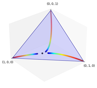
This black dot is the stationary distribution \(\psi^*\) of the Markov semigroup \((P_t)\) generated by \(Q\).
It was calculated using the stationary_distributions attribute of QuantEcon’s
MarkovChain class, by arbitrarily setting \(t=1\) and solving \(\psi P_1 = \psi\).
Below we show that, for this choice of \(Q\), the stationary distribution \(\psi^*\) is unique in \(\dD\), due to irreducibility.
Moreover, \(\psi P_t \to \psi^*\) as \(t \to \infty\) for any \(\psi \in \dD\), as suggested by the figure.
8.2.2. Stationarity via the Generator
In many cases, it is easier to use the generator of the semigroup to identify stationary distributions rather than the semigroup itself.
This is analogous to the idea that a point \(\bar x\) in \(\RR^d\) is stationary for a vector ODE \(x'_t = F(x_t)\) when \(F(\bar x) = 0\).
(Here \(F\) is the infinitesimal description, and hence analogous to the generator.)
The next result holds true under weaker conditions but the version stated here is easy to prove and sufficient for applications we consider.
Theorem 8.1
Let \((P_t)\) be a UC Markov semigroup with generator \(Q\). A distribution \(\psi\) on \(S\) is stationary for \((P_t)\) if and only if \(\psi Q = 0\).
Proof. Fix \(\psi \in \dD\) and suppose first that \(\psi Q = 0\).
Since \((P_t)\) is a UC Markov semigroup, we have \(P_t = e^{tQ}\) for all \(t\), and hence, for any \(t \geq 0\),
From \(\psi Q = 0\) we get \(\psi Q^k = 0\) for all \(k \in \NN\), so the last display yields \(\psi P_t = \psi\).
Hence \(\psi\) is stationary for \((P_t)\).
Now suppose that \(\psi\) is stationary for \((P_t)\) and set \(D_t := (1/t) (P_t - I)\).
From the triangle inequality and the definition of the operator norm, for any given \(t\),
Since \((P_t)\) is UC and \(Q\) is its generator, we have \(\| D_t - Q \| \to 0\) in \(\lL(\ell_1)\) as \(t \to 0^+\).
Hence \(\| \psi Q \| \leq \liminf_{t \downarrow 0} \| \psi D_t \|\).
As \(\psi\) is stationary for \((P_t)\), we have \(\psi D_t = 0\) for all \(t\).
Hence \(\psi Q = 0\), as was to be shown.
8.3. Irreducibility and Uniqueness
Let \((P_t)\) be a Markov semigroup on \(S\) and consider arbitrary states \(x, y \in S\).
We say that state \(y\) is accessible from state \(x\) if there exists a \(t \geq 0\) such that \(P_t(x, y) > 0\).
We say that \(x\) and \(y\) communicate if \(x\) is accessible from \(y\) and \(y\) is accessible from \(x\).
A Markov semigroup \((P_t)\) on \(S\) is called irreducible if every pair \(x,y\) in \(S\) communicates.
We seek a characterization of irreducibility of \((P_t)\) in terms of its generator.
As a first step, we will say there is a \(Q\)-positive probability flow from \(x\) to \(y\) if there exists a finite sequence \((z_i)_{i=0}^m\) in \(S\) starting at \(x=z_0\) and ending at \(y=z_m\) such that \(Q(z_i, z_{i+1}) > 0\) for all \(i\).
Theorem 8.2
Let \((P_t)\) be a UC Markov semigroup with generator \(Q\). For distinct states \(x\) and \(y\), the following statements are equivalent:
The state \(y\) is accessible from \(x\) under \((P_t)\).
There is a \(Q\)-positive probability flow from \(x\) to \(y\).
\(P_t(x, y) > 0\) for all \(t > 0\).
Proof. Pick any two distinct states \(x\) and \(y\).
It is obvious that statement 3 implies statement 1, so we need only prove (1 \(\implies\) 2) and (2 \(\implies\) 3).
Starting with (1 \(\implies\) 2), recall that
If \(x\) is accessible from \(y\), then \(P_t(x, y) > 0\) for some \(t > 0\), so \(Q^k(x,y) > 0\) for at least one \(k \in \NN\).
Writing out the matrix product as a sum, we now have
It follows that at least one element of the sum must be strictly positive.
Therefore, a \(Q\)-positive probability flow from \(x\) to \(y\) exists.
Turning to (2 \(\implies\) 3), first note that, for arbitrary states \(u\) and \(v\), if \(Q(u, v) > 0\) then \(P_t(u, v) > 0\) for all \(t > 0\).
To see this, let \((\lambda, K)\) be the jump chain pair constructed from \(Q\) via (7.8), (7.9) and (7.10).
Observe that, since \(Q(u, v) > 0\), we must have \(\lambda(u) > 0\).
As a consequence, applying (7.10), we have
Let \((Y_k)\) and \((J_k)\) be the embedded jump chain and jump sequence generated by Algorithm 4.1, with \(Y_0 = u\).
With \(E_1 \sim \Exp(1)\) and \(E_2 \sim \Exp(1)\), we have, for any \(t > 0\),
Now suppose there is a \(Q\)-positive probability flow \((z_i)_{i=0}^m\) from \(x\) to \(y\).
If we fix \(t > 0\) and repeatedly apply (3.7) along with the last result, we obtain
Theorem 8.2 leads directly to the following strong result.
Corollary 8.1
For a UC Markov semigroup \((P_t)\), the following statements are equivalent:
\((P_t)\) is irreducible.
\(P_t(x,y) > 0\) for all \(t > 0\) and all \((x,y) \in S \times S\).
Note
To obtain stable long run behavior in discrete time Markov chains, it is common to assume that the chain is aperiodic.
This needs to be assumed on top of irreducibility if one wishes to rule out all dependence on initial conditions.
Corollary 8.1 shows that periodicity is not a concern for irreducible continuous time Markov chains.
Positive probability flow from \(x\) to \(y\) at some \(t > 0\) immediately implies positive flow for all \(t > 0\).
8.4. Asymptotic Stabilitiy
We call Markov semigroup \((P_t)\) asymptotically stable if \((P_t)\) has a unique stationary distribution \(\psi^*\) in \(\dD\) and
Our aim is to establish conditions for asymptotic stability of Markov semigroups.
8.4.1. Contractivity
Let’s recall some useful facts about the discrete time case.
First, if \(P\) is any Markov matrix, we have, in the \(\ell_1\) norm,
This is because, given \(\psi \in \dD\),
By linearity, for \(\psi, \phi \in \dD\), we then have
Hence every Markov operator is contracting on \(\dD\).
Moreover, if \(P\) is everywhere positive, then this inequality is strict:
Lemma 8.1 (Strict Contractivity)
If \(P\) is a Markov matrix and \(P(x, y) > 0\) for all \(x, y\), then
The proof follows from the strict triangle inequality, as opposed to the weak triangle inequality we used to obtain (8.4).
See, for example, Proposition 3.1.2 of [Lasota and Mackey, 1994] or Lemma 8.2.3 of [Stachurski, 2009].
8.4.2. Uniqueness
Irreducibility of a given Markov chain implies that there are no disjoint absorbing sets.
This in turn leads to uniqueness of stationary distributions:
Theorem 8.3
Let \((P_t)\) be a UC Markov semigroup on \(S\). If \((P_t)\) is irreducible, then \((P_t)\) has at most one stationary distribution.
Proof. Suppose to the contrary that \(\psi\) and \(\phi\) are both stationary for \((P_t)\).
Since \((P_t)\) is irreducible, we know that \(P_1(x,y) > 0\) for all \(x,y \in S\).
If \(\psi \not= \phi\), then, due to positivity of \(P_1\), the strict inequality in Lemma 8.1 holds.
At the same time, by stationarity, \(\| \psi P - \phi P \| = \| \psi - \phi \|\). Contradiction.
Example 8.1
An M/M/1 queue with parameters \(\mu, \lambda\) is a continuous time Markov chain \((X_t)\) on \(S = \ZZ_+\) with with intensity matrix
The chain \((X_t)\) records the length of the queue at each moment in time.
The intensity matrix captures the idea that customers flow into the queue at rate \(\lambda\) and are served (and hence leave the queue) at rate \(\mu\).
If \(\lambda\) and \(\mu\) are both positive, then there is a \(Q\)-positive probability flow between any two states, in both directions, so the corresponding semigroup \((P_t)\) is irreducible.
Theorem 8.3 now tells us that \((P_t)\) has at most one stationary distribution.
8.4.3. Stability from the Skeleton
Recall the definition of asymptotic stability given in (8.3).
Analogously, we call an individual Markov operator \(P\) asymptotically stable if \(P\) has a unique stationary distribution \(\psi^*\) in \(\dD\) and \(\psi P^n \to \psi^*\) as \(n \to \infty\) for all \(\psi \in \dD\).
The next result gives a connection between discrete and continuous stability.
The critical ingredient linking these two concepts is the contractivity in (8.4).
Lemma 8.2
Let \((P_t)\) be a Markov semigroup. If there exists an \(s > 0\) such that the Markov matrix \(P_s\) is asymptotically stable, then \((P_t)\) is asymptotically stable with the same stationary distribution.
Proof. Let \((P_t)\) and \(s\) be as in the statement of Lemma 8.2.
Let \(\psi^*\) be the stationary distribution of \(P_s\). Fix \(\psi \in \dD\) and \(\epsilon > 0\).
By stability of \(P_s\), we can take an \(n \in \NN\) such that \(\| \psi P_s^n - \psi^* \| < \epsilon\).
Pick any \(t > sn\). Set \(h := t - sn\).
By the contractivity in (8.4) and \(P_{sn} = P_s^n\), we have
Hence asymptotic stability holds for \((P_t)\).
8.4.4. Stability via Drift
In this section we address drift conditions, which are a powerful method for obtaining asymptotic stability when the state space can be infinite.
The idea is to show that the state tends to drift back to a finite set over time.
Such drift, when combined with the contractivity in Lemma 8.1, is enough to give global stability.
The next theorem gives a useful version of this class of results.
Theorem 8.4
Let \((P_t)\) be a UC Markov semigroup with intensity matrix \(Q\). If \((P_t)\) is irreducible and there exists a function \(v \colon S \to \RR_+\), a finite set \(F \subset S\) and positive constants \(\epsilon\) and \(M\) such that
then \((P_t)\) is asymptotically stable.
The proof of Theorem 8.4 can be found in [Pichór et al., 2012].
Example 8.2
Consider again the M/M/1 queue on \(\ZZ_+\) with intensity matrix (8.5).
Suppose that \(\lambda < \mu\).
It is intuitive that, in this case, the queue length will not tend to infinity (since the service rate is higher than the arrival rate).
This intuition can be confirmed via Theorem 8.4, after setting \(v(j) = j\).
Indeed, we have, for any \(i \geq 1\),
Setting \(F=\{0\}\) and \(M = \lambda - \mu = - \epsilon\), we see that the conditions of Theorem 8.4 hold.
Hence the associated semigroup \((P_t)\) is asymptotically stable.
Corollary 8.2
If \((P_t)\) is an irreducible UC Markov semigroup and \(S\) is finite, then \((P_t)\) is asymptotically stable.
A solved exercise below asks you to confirm this.
8.5. Exercises
Exercise 8.1
Let \((P_t)\) be a Markov semigroup. True or false: for this semigroup, every state \(x\) is accessible from itself.
Exercise 8.2
Let \((\lambda_k)\) be a bounded non-increasing sequence in \((0, \infty)\).
A pure birth process starting at zero is a continuous time Markov process \((X_t)\) on state space \(\ZZ_+\) with intensity matrix
Show that \((P_t)\), the corresponding Markov semigroup, has no stationary distribution.
Exercise 8.3
Confirm that Theorem 8.4 implies Corollary 8.2.
8.6. Solutions
Suppose to the contrary that \(\phi \in \dD\) and \(\phi Q = 0\).
Then, for any \(j \geq 1\),
Since \((\lambda_k)\) is non-increasing, it follows that
Therefore, for any \(j\geq 1\), it must be:
It follows that \(\phi\) is non-decreasing on \(\ZZ_+\).
But \(\dD\) contains no non-decreasing functions when the state space is infinite. (Why?)
Contradiction.
Let \((P_t)\) be an irreducible UC Markov semigroup and let \(S\) be finite.
Pick any positive constants \(M, \epsilon\) and set \(v = M\) and \(F = S\).
We then have
Hence the drift condition in Theorem 8.4 holds and \((P_t)\) is asymptotically stable.